CSC/ECE 506 Spring 2010/ch 2 aj/Data Parallel Programming
Data-Parallel Programming Model
Introduction
Data-parallel processing is when multiple processing elements perform an action separately on different sets of data and exchange information globally before processing more code synchronously. Even though this model is offered in contrast to the shared memory model and the message passing model, data-parallel processing can be accomplished by actually passing messages or sharing memory at a deeper level. The main distinction between the data-parallel model and the other two models has to do with the outcome of the individual steps instead of the method of communication.
Data-parallel processing has been found to be effective in situations where computations involve every element of a matrix in a uniform way. This allows the processing to be divided spatially over memories. Originally, the need for this model was discovered in scientific calculations and is still used today.
Data parallelism vs Task parallelism
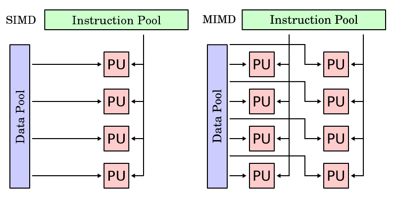
One important feature of data parallel programming model or data parallelism (SIMD) is the single control flow: there is only one control processor that directs the activities of all the processing elements. In stark contrast to this is task parallelism (MIMD): characterized by its multiply control flow, it allows the concurrent execution of multiply instruction stream, each manipulating its own data and servicing separate functions. Below are contrast of SIMD and MIMD model form wikipedia pages of SIMD and MIMD.

Synchronous vs Asynchronous
While data parallelism's single control over all processing elements ensures synchronous computation, every processor in task parallelism performs its task in their own pace, which we call asynchronous computation. Thus, at certain point of the execution of a task parallel program, communication and synchronization primitives are needed to allow different instruction streams to coordinate their efforts.
Example
This section shows a simple example adapted from Solihin textbook (pp. 24 - 27) that illustrates the data-parallel programming model. Each of the codes below are written in pseudo-code style.
Suppose we want to perform the following task on an array a: updating each element of a by the product of itself and its index, and adding together the elements of a into the variable sum. The corresponding code is shown below.
// simple sequential task
sum = 0;
for (i = 0; i < a.length; i++)
{
   a[i] = a[i] * i;
   sum = sum + a[i];
}
When we implement the task using the data-parallel programming model, the program can be divided into two parts. The first part performs the same operations on separate elements of the array for each processing element (sometimes referred to as PE or pe), and the second part reorganizes data among all processing elements (In our example data reorganization is summing up values across different processing elements). Since data-parallel programming model only defines the overall effects of parallel steps, the second part can be accomplished either through shared memory or message passing. The three code fragments below are examples for the first part of the program, shared-memory version of the second part, and message passing for the second part, respectively.
// data parallel programming: let each PE perform the same task on different pieces of distributed data
pe_id = getid();
my_sum = 0;
for (i = pe_id; i < a.length; i += number_of_pe)         //separate elements of the array are assigned to each PE
{
   a[i] = a[i] * i;
   my_sum = my_sum + a[i];                               //all PEs accumulate elements assigned to them into local variable my_sum
}
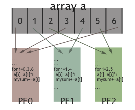
In the above code, data parallelism is achieved by letting each processing element perform actions on array's separate elements, which are identified using the PE's id. For instance, if three processing elements are used then one processing element would start at i = 0, one would start at i = 1, and the last would start at i = 2. Since there are three processing elements then the index of the array for each will increase by three on each iteration until the task is complete (note that in our example elements assigned to each PE are interleaved instead of continuous). If the length of the array is a multiple of three then each processing element takes the same amount of time to execute its portion of the task.
.The picture below illustrates how elements of the array are assigned among different PEs for the specific case: length of the array is 7 and there are 3 PEs available. Elements in the array are marked by their indexes(0 to 6). As shown in the picture, PE0 will work on elements with index 0, 3, 6; PE1 is in charge of elements with index 1, 4; and elements with index 2, 5 are assigned to PE2. In this way, these 3 PEs work collectively on the array, while each PE works on different elements. Thus, data parallelism is achieved.

Other Parallel Programming Models
Example continued
As previously mentioned, the shared memory and message passing parallel programming models are commonly used. The following descriptions and code snippets are intended to develop a contrast between the data-parallel programming model and the other two models.
The code below shows how data reorganization is done by the shared memory programming model. A shared variable is declared to store the global sum. Each PE accumulates their local my_sum into this variable. In this example, the lock() and unlock() routines are used to prevent race conditions and barrier ensures that the all the local my_sum variables have been accumulated into the shared variable sum before the code proceeds. Notice that in this model there is only one copy of the data like in the data-parallel model. However, in the shared memory model, the data must be protected since any PE could be using it at any point, whereas data is associated with a specific PE in the data-parallel model.
// data reorganization via shared memory
shared sum;
lock();                                                  //prevent race condition
sum = sum + my_sum;                                      //each PE adds up their local my_sum to shared variable sum
unlock();
barrier;
The final section of code shows how data reorganization is done by the message passing programming model. PE0 acts as the one that collects the local my_sum variable from all the other PEs. This is done by the send_msg() and the recv_msg() routines: PEs other than PE0 send their my_sum variable as a message to PE0. PE0 receives the messages by specifying the sender in the for loop. PE ids are used in the message passing model in the same way they are in the data-parallel model. On the contrary, in the data-parallel model there is only one copy of data that is processed and there is no need to do any final accumulation by a single PE.
// data reorganization via message passing
if (pe_id != 0) send_msg (0, my_sum);                    //PE other than PE0 send their local my_sum
else                                                     //PE0 does this
{
   for (i = 1; i < number_of_pe; i++)                    //for each other PE
   {
      recv_msg (i, temp);                                //receive local sum from other PEs
      my_sum = my_sum + temp;                            //accumulate into total
   }
   sum = my_sum;
}
Comparison in different aspects
The table below is extended from Table 2.1 on page 22 of the Solihin text. A column has been added for the data-parallel model. The table compares some key characteristics of each programming model. As you can see, the complexity of the data-parallel model comes mainly in the form of dividing up the work among PEs. Most of this work is done by the programmer and does not necessarily require special hardware, although, specific types of hardware can optimize the benefits of the model. For instance, SIMD and SPMD hardware are examples that have efficiently utilized the data-parallel model.
| Aspects | Data-Parallel | Shared Memory | Message Passing |
|---|---|---|---|
| Communication | implicit - via loads/stores | implicit - via loads/stores | explicit messages |
| Synchronization | none | explicit | implicit - via messages |
| Hardware support | none | typically required | none |
| Development effort | low | low | high |
| Tuning effort | high | high | low |
Recent changes
As mentioned previously, the data-parallel programming model in itself is a contrast to the shared memory programming model and the message passing programming model. Now, with the evolution of SIMD to single-program-multiple data (SPMD) machines, multiple processing elements run identical copies of the same program. In addition, SPMD now indeed uses a form of shared memory and message-passing to communicate between processing elements. As a result, even though each of the three parallel programming models have distinct features, it appears the trends are for a convergence that integrates multiple models into a single system.
References
1) David E. Culler, Jaswinder Pal Singh, and Anoop Gupta, Parallel Computer Architecture: A Hardware/Software Approach, Gulf Professional Publishing, August 1998.
2) Yan Solihin, Fundamentals of Parallel Computer Architecture: Multichip and Multicore Systems, Solihin Books, August 2009.
3) Philip J. Hatcher, Michael Jay Quinn, Data-Parallel Programming on MIMD Computers, The MIT Press, 1991.
4) Blaise Barney, "Introduction to Parallel Computing: Data Parallel Model", Lawrence Livermore National Laboratory, https://computing.llnl.gov/tutorials/parallel_comp/#ModelsData, January 2009.