CSC/ECE 506 Spring 2011/ch4a zz: Difference between revisions
| Line 33: | Line 33: | ||
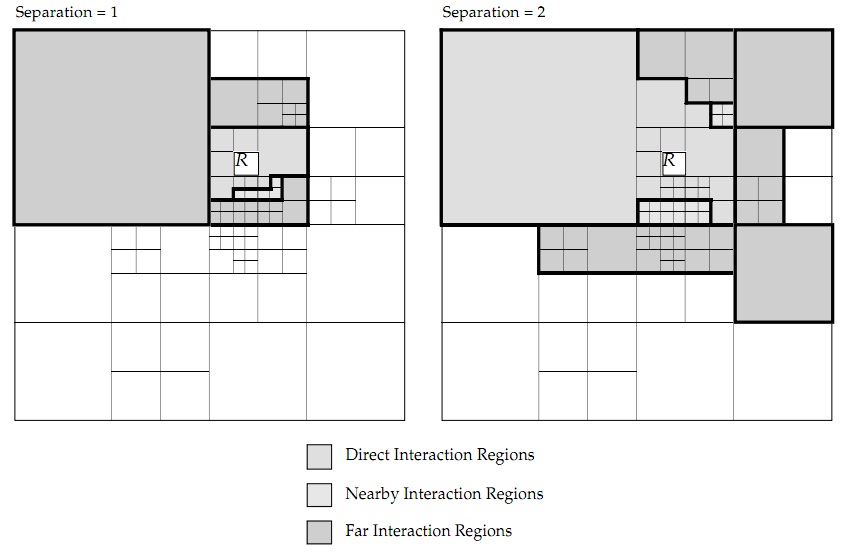
[[Image: data.jpg|frame|center|Adaptive decompositions for a given box R, showing examples for separations of 1 and 2. Figure from [6]]] | [[Image: data.jpg|frame|center|Adaptive decompositions for a given box R, showing examples for separations of 1 and 2. Figure from [6]]] | ||
By separating the blocks by the Hamming distance to the R block. Three interaction list could be created by the distance: The direct interaction list ''D''''r''; the far interaction list ''F''''r'' and the intermediate interaction list ''H''''r'' | |||
The steps for each iteration using the given decomposition of the simulation are: | |||
<pre> | |||
1. Compute the multipole expansion coefficients for all leaves in the tree decomposition. | |||
2. Compute the multipole expansion coefficients for all internal nodes in the tree with depth ≥ 2. | |||
3. Compute the local expansion coefficients for a region R by summing R’s parent’s local expansion (shifted from the parent’s center to the center of R) with the sum of all of the multipole | |||
expansions in R’s far list, FR (converting the multipole expansions to local expansions and shifting to the center of R) for all regions with depth ≥ 2. | |||
4. For each body, b, in each leaf region, R, compute all the direct forces on b from all the bodies in the regions in R’s direct interaction list (DR). | |||
5. For each body, b, in each leaf region, R, compute the far force on b by evaluating the local expansion for region R at b’s position. | |||
6. For each body, b, in each leaf region, R, compute the intermediate force by evaluating the multipole expansion at b’s position for each region in R’s intermediate interaction list (HR). | |||
7. Sum the 3 components of the force and potential | |||
for each body. | |||
8. Apply the forces, updating the positions and velocities, and move the bodies to their proper regions as indicated by boundary crossing. | |||
</pre> | |||
=== shared-memory === | === shared-memory === | ||
Revision as of 04:49, 28 February 2011
Introduction

The N-body problem stated as follows: Select the position and velocity of n celestial bodies as states. Given the initial condition of of N bodies, compute their states at arbitrary time T. Normally a three-dimensional space is considered for N-body problem. There is a simplified N-body problem called restricted N-body problem where the mass of some of the bodies is negligible. Several remarkable three-body simulation can be found in [1].

Many mathematicians have proofed that it is impossible to find a general solution for n-body problem analytically[2][3]. The system could become unstable very easily. However, the problem can be solved numerically. The most common approach is to iterate over a sequence of small time steps. Within each time step, the acceleration on a body is approximated by the transient acceleration in the pervious time step. The transient acceleration on a single body can be directly computed by summing the gravity from each of the other N-1 bodies. While this method is conceptually simple and is the algorithm of choice for many applications, its O(N2)
The simulation of N-body system can be used from simulation of celestial bodies (gravitational interaction)to interactions of a set of particles (electromagnetic interaction).
Parallel N-body problem

Since each particle will interact with others by the force of gravity, the simulation of N-body system is computationally expensive for large numbers of N. There a O(N2) interactions to compute for every iteration. Furthermore, in order to have a accurate result, the discrete time step must relatively small. Thus, there has been a huge interest in faster parallel algorithm for N-body problem.
Early parallel algorithms
In 1985, Appel took the first step of decomposes the problem by introducing a tree structure[4]. In the next year, Barnes and Hut extend the tree-based force calculation with logarithmic growth of force terms per particle[5]. The partition is shown on the left. The empty block have been pruned, thus the traversal time have been reduced fromO(N2) to O(N logN).
For each time step:
1. Build the BH tree.
2. Compute centers-of-mass bottom-up
3. For each body
   Star a depth-first traversal of the tree;
   Truncating the search at internal nodes where the approximation is applicable;
   Update the contribution of the node to the acceleration of the body.
4. Update the velocity and position of each body.
data-parallel

By separating the blocks by the Hamming distance to the R block. Three interaction list could be created by the distance: The direct interaction list D'r; the far interaction list F'r and the intermediate interaction list H'r
The steps for each iteration using the given decomposition of the simulation are:
1. Compute the multipole expansion coefficients for all leaves in the tree decomposition.
2. Compute the multipole expansion coefficients for all internal nodes in the tree with depth ≥ 2.
3. Compute the local expansion coefficients for a region R  by summing R’s parent’s local expansion (shifted from the parent’s center to the center of R) with the sum of all of the multipole
expansions in R’s far list, FR (converting the multipole expansions to local expansions and shifting to the center of R) for all regions with depth ≥ 2.
4. For each body, b, in each leaf region, R, compute all the direct forces on b from all the bodies in the regions in R’s direct interaction list (DR).
5. For each body, b, in each leaf region, R, compute the far force on b by evaluating the local expansion for region R at b’s position.
6. For each body, b, in each leaf region, R, compute the intermediate force by evaluating the multipole expansion at b’s position for each region in R’s intermediate interaction list (HR).
7. Sum the 3 components of the force and potential
for each body.
8. Apply the forces, updating the positions and velocities, and move the bodies to their proper regions as indicated by boundary crossing.
message-passing
References
[1] [1] Collection of remarkable three-body motions
[2][[2]] something about Poincaré
[3] Diacu, F (01/01/1996). "The solution of the n-body problem". The Mathematical intelligencer (0343-6993), 18 (3), p. 66.
[4] A. Appel, "An Efficient Program for Many-Body Simulation", SIAM J. Scientific and Statistical Computing, vol. 6, 1985
[5] Barnes. Josh, Hut. Piet, (12/04/1986). "A hierarchical O(N log N) force-calculation algorithm". Nature (London) (0028-0836), 324 (6096), p. 446.
[6] A Data-Parallel Implementation of the Adaptive Fast Multipole Algorithm 1993