CSC/ECE 506 Spring 2011/ch4a zz: Difference between revisions
No edit summary |
|||
| (269 intermediate revisions by the same user not shown) | |||
| Line 1: | Line 1: | ||
= | = Introduction = | ||
[[Image: | [[Image:Nasanbody.jpg|thumb|left|N-body Problem. Picture source: NASA]] | ||
[[ | N-body problem is one of the most important topics in [http://en.wikipedia.org/wiki/Celestial_mechanics celestial mechanics]. The [http://en.wikipedia.org/wiki/N-body_problem#Mathematical_formulation_of_the_n-body_problem mathematical formulation of N-body problem] is a little bit beyond the scope of this book so it will not be discussed here. Based on the mathematics, we can simplify the N-body problem as follows: Select the position and velocity of N celestial bodies as [http://en.wikipedia.org/wiki/State_space_%28controls%29#State_variables state variables]. Given the [http://en.wikipedia.org/wiki/Initial_value_problem initial condition] of N bodies, compute their states at arbitrary time T. Normally a three-dimensional space is considered for N-body problem. There is a simplified N-body problem called restricted N-body problem where the mass of some of the bodies is negligible. Several remarkable three-body simulation can be found in [[#References|[1]]]. | ||
[ | |||
[[Image:3body.png|thumb|right|The trajectory of restricted three-body system [[#References|[1]]] ]] | |||
The | Many mathematicians have proofed that it is impossible to find a [http://en.wikipedia.org/wiki/Closed-form_expression closed-form solution] for n-body problem analytically[[#References|[2]]][[#References|[3]]]. The system could become [http://www.scholarpedia.org/article/Stability unstable] very easily. However, the problem can be solved [http://en.wikipedia.org/wiki/Numerical_analysis numerically]. The most common approach is to iterate over a sequence of small time steps. Within each time step, the acceleration on a body is approximated by the transient acceleration in the previous time step. The transient acceleration on a single body can be directly computed by summing the gravity from each of the other N-1 bodies. While this method is conceptually simple and is the algorithm of choice for many applications, its ''O''(''N''<sup>2</sup>). | ||
The | The simulation of N-body system can be used from simulation of celestial bodies ([http://www.mpa-garching.mpg.de/galform/virgo/millennium/index.shtml gravitational interaction])to interactions of a set of particles (electromagnetic interaction). | ||
= Parallel N-body problem = | |||
As MIT professors Dimitri Bertsekas and John Tsitsiklis stated in their book [http://web.mit.edu/dimitrib/www/pdc.html "Parallel and Distributed Computation: Numerical Methods"], parallel computers have provided an excellent platform for numerical analysis. In the N-body problem, since each particle will interact with others by the force of gravity, the simulation of N-body system is computationally expensive for large numbers of N. There a ''O''(''N''<sup>2</sup>) interactions to compute for every iteration. Furthermore, in order to have a accurate result, the discrete time step must relatively small. Thus, there has been a huge interest in faster parallel algorithm for N-body problem. | |||
== Data-parallel Implementation == | |||
=== Barnes-Hut Tree (BH tree) === | |||
In 1985, Appel took the first step of decomposes the problem by introducing a tree structure[[#References|[4]]]. In the next year, Barnes and Hut extend the tree-based force calculation with logarithmic growth of force terms per particle[[#References|[5]]]. That is, construct a tree hierarchy(BH tree) of bodies based on the partition of entire space. The partition is shown on the left. The empty block have been pruned, thus the traversal time have been reduced from''O''(''N''<sup>2</sup>) to ''O''(''N'' log''N''). | |||
[[Image:BHtree.jpg|center|frame|A recursive partition in two dimension and its corresponding BH tree. Picture from [[#References|[6]]] ]] | |||
<pre> | |||
For each time step: | |||
1. Build the BH tree. | |||
2. Compute centers-of-mass bottom-up | |||
3. For each body | |||
Star a depth-first traversal of the tree; | |||
Truncating the search at internal nodes where the approximation is applicable; | |||
Update the contribution of the node to the acceleration of the body. | |||
4. Update the velocity and position of each body. | |||
</pre> | |||
There are several challenges of this decomposition: | |||
# Unlike the ocean current can be represented evenly by regular grid points in the entire space, the density of the galaxies is varying in different space. In some spaces the density of stars maybe very high, but in some other spaces there might be only few stars at certain time. This implies the computation load for each body will be different. | |||
# The other challenge is that the position of the body is time-varying, which means the static assignment (which has been used in ocean application) may not work well. | |||
# The force calculation of certain a body needs information from other bodies. In order to reduce the communication among processors, the partitions needs to be contiguous in any directions. | |||
# The last challenge is that there is a trade-off between the level of decomposition and communication. That is, the fine grained approach could speed-up the force calculation but it will need more communications between different groups of stars. | |||
Even though the Barnes-Hut tree decomposition algorithm have these challenges, BH tree is still the one of most efficient methods for solving the n-body problem. | |||
=== Orthogonal Recursive Bisection (ORB) === | |||
[[Image: orthogonal recursive bisection.gif|right|frame|upright=0.5| [http://en.wikipedia.org/wiki/CUDA Orthogonal Recursive Bisection] ]] | |||
Unlike BH tree divided the space into square cells, the Orthogonal Recursive Bisection (ORB) divided space into rectangular with same number of bodies in each of them. It is a recursive approach because all processors are associated with the entire space at the very beginning; then a orthogonal line has been drawn to separate the space into bisection; each of the subsection has associated with half of the processors. Until the number of partition is equal to the number of processors. | |||
=== Other Data-parallel Implementation === | |||
When using data-parallel algorithm to solve the N-body problem, one obvious approach for the data-parallel implementation is to divide the interactions into different sets based on the distances from current particle to other "interacting" particles. Thus the force from 'far away' particles can be updated less frequently or even can be ignored. | |||
[[Image: data.jpg|thumb|left|Adaptive decompositions for a given box R, showing examples for separations of 1 and 2. Figure from [[#References|[6]]] ]] | |||
By separating the blocks by the Hamming distance to the R block. Three interaction list could be created by the distance: The direct interaction list ''Dr''; the far interaction list ''Fr'' and the intermediate interaction list ''Hr'' | |||
The steps for each iteration using the given decomposition of the simulation are [[#References|[6]]]: | |||
# Compute the multipole expansion coefficients for all leaves in the tree decomposition. | |||
# Compute the multipole expansion coefficients for all internal nodes in the tree with depth ≥ 2. | |||
# Compute the local expansion coefficients for a region R by summing R’s parent’s local expansion (shifted from the parent’s center to the center of R) with the sum of all of the multipole expansions in R’s far list, ''Fr''(converting the multipole expansions to local expansions and shifting to the center of R) for all regions with depth ≥ 2. | |||
# For each body, b, in each leaf region, R, compute all the direct forces on b from all the bodies in the regions in R’s direct interaction list (''Dr''). | |||
# For each body, b, in each leaf region, R, compute the far force on b by evaluating the local expansion for region R at b’s position. | |||
# For each body, b, in each leaf region, R, compute the intermediate force by evaluating the multipole expansion at b’s position for each region in R’s intermediate interaction list (''Hr''). | |||
# Sum the 3 components of the force and potential for each body. | |||
# Apply the forces, updating the positions and velocities, and move the bodies to their proper regions as indicated by boundary crossing. | |||
Another data-parallel implementation can be found in [[#References|[8]]]. The drawback of this type of approach is obvious: the error may be increased significantly due to the clustering process. | |||
== Shared-memory Implementation == | |||
=== Costzones === | |||
[[Image: Costzone.png|center|frame| [http://www.eecs.berkeley.edu/~demmel/cs267/lecture27/lecture27.html The partitioning of Costzones] ]] | |||
It is easy to share the BH tree in a shared memory machine. The so-called Costzones is one of the approaches to implement the BH tree algorithm in the shared-memory machine. We know that the processor will accesses more the nearby bodies than distant ones. Since the BH tree already contain the spatial information of bodies (more likely the nearby bodies will have a same parent with me), the Costzones technique simply uses the data structure created by the BH tree. | |||
The costzones method have a better performance in a shared-memory machine compared with the ORB method. The reason is mainly because the time spent in the space partition is shorter. | |||
=== Other Shared-memory Implementation === | |||
Besides the Costzones method of implementing the N-body simulation on shard-memory machines, there is a tremendous interests of using [http://en.wikipedia.org/wiki/CUDA CUDA] to solve the N-body problem by modern GPUs [[#References|[10]]][[#References|[11]]]. | |||
<pre> | |||
global void | |||
calculate_forces(void *devX, void *devA) | |||
{ | |||
extern __shared__ float4[] shPosition; | |||
float4 *globalX = (float4 *)devX; | |||
float4 *globalA = (float4 *)devA; | |||
float4 myPosition; | |||
int i, tile; | |||
float3 acc = {0.0f, 0.0f, 0.0f}; | |||
int gtid = blockIdx.x * blockDim.x + threadIdx.x; | |||
myPosition = globalX[gtid]; | |||
for (i = 0, tile = 0; i < N; i += p, tile++) { | |||
int idx = tile * blockDim.x + threadIdx.x; | |||
shPosition[threadIdx.x] = globalX[idx]; | |||
syncthreads(); | |||
acc = tile_calculation(myPosition, acc); | |||
syncthreads(); | |||
} | |||
// Save the result in global memory for the integration step. | |||
float4 acc4 = {acc.x, acc.y, acc.z, 0.0f}; | |||
globalA[gtid] = acc4; | |||
} | |||
</pre> | |||
CUDA shows an impressive potential to execute extremely parallel applications such as N-body problem. Twenty years ago, the N-body simulation can only runs on super computers. Because of the development of CUDA makes the classical N-body problem become a term project for some graduate students (see [http://www.evl.uic.edu/sjames/cs525/project2.html 2008 Fall CS 525 Project2 n-body simulation in CUDA]). | |||
== Message-passing Implementation == | |||
[[Image: Octtree.png|frame|right|A quad-tree shown along with the binary key coordinates of the nodes. Figure from [[#References|[9]]] ]] | |||
Implementing the BH tree algorithm is more difficult in a distributed-memory system compared with the shared-memory implementation. Because we need assign the different bodies to different processor dynamically. When the location of bodies have been changed exceed a certain limit, the BH tree needs to be reconstruct. The good news is we don't need reconstruct the BH tree very frequently(compared with the simulation step size). | |||
In message-passing architectures, a processor’s local memory is often used as a software-controlled cache | |||
for communicated data, in addition to holding the processor’s own assigned data partition; that is, data are replicated in the memories of those processors that need to use them. | |||
Warren and Salmon introduced a parallel hashed Oct-tree N-body algorithm[[#References|[9]]]. The hashed Oct-tree is the message-passing version of BH tree implementation. One of the advantages of using hash table is that the non-local data may be accessed by requesting a key, which is a uniform addressing scheme and easy to be implemented on a message passing architecture. The pseudocode of tree traversal are shown below: | |||
<pre> | |||
ListTraverse((*MAC)(hcell *)) | |||
{ | |||
copy root to walk_list; | |||
while (!Empty(walk_list)) { | |||
for (each item on walk_list) { | |||
for (each daughter of item) { | |||
if (MAC(daughter)) | |||
copy daughter to interact_list; | |||
else | |||
copy daughter to output_walk_list; | |||
} | |||
} | |||
walk_list = output_walk_list; | |||
} | |||
} | |||
</pre> | |||
There are two major challenges of using message-passing parallel to solve the N-body problem: | |||
# The nonuniform and dynamic nature of the particle distribution, which implies that the partitions assigned to processors change with time to maintain load balancing and data locality; | |||
# The need for long-range communication which is irregular as a result of the nonuniformity. | |||
The typical message-passing strategy of allowing communicated data to accumulate in local memory and flushing them out at | |||
certain points in the program does not work well here like it does in regular predictable programs. Thus, the only convenient points at which to flush communicated data in the application program are the boundaries between computational phases. Since the amount of nonlocal data read from the tree during the force computation phase can be quite large, the memory overhead due to data replication can be large when replacement is managed in this typical message-passing style. | |||
== Other Parallel Approaches == | |||
Other than the conventional approaches, there are also some new techniques have been developed to simulate the N-body problem: | |||
* Hardware side: The researcher in University of Tokyo have designed and built a special purpose hardware called GRAPE for the N-body simulation. The chip has been designed to optimize the computation of gravitational interactions.[[#References|[12]]] The GRAPE has been keep developed by researchers, the most updated version is [http://adsabs.harvard.edu/abs/2003PASJ...55.1163M GRAPE 6]. | |||
* Software (algorithm) side: On the other hand, the high-level architecture-independent algorithms also have been develop to simulate the N-body problem[[#References|[13]]]. These algorithm allowed researchers test their prototype parallel program under different architecture without using the machine-specified languages. | |||
=References= | |||
[1] [http://faculty.ifmo.ru/butikov/Projects/Collection1.html Collection of remarkable three-body motions] | |||
[2] [http://en.wikipedia.org/wiki/Henri_Poincar%C3%A9 About Henri Poincaré] | |||
[3] Diacu, F (01/01/1996). [http://rutherglen.science.mq.edu.au/math332s207/diacuNbody.pdf "The solution of the n-body problem"] . The Mathematical intelligencer (0343-6993), 18 (3), p. 66. | |||
[4] A. Appel, [http://epubs.siam.org.www.lib.ncsu.edu:2048/sisc/resource/1/sjoce3/v6/i1/p85_s1 "An Efficient Program for Many-Body Simulation"] , SIAM J. Scientific and Statistical Computing, vol. 6, 1985 (available at NCSU library) | |||
[5] Barnes. Josh, Hut. Piet, (12/04/1986). [http://www.nature.com.www.lib.ncsu.edu:2048/nature/journal/v324/n6096/abs/324446a0.html "A hierarchical O(N log N) force-calculation algorithm".] Nature (London) (0028-0836), 324 (6096), p. 446. (available at NCSU library) | |||
[6] [http://citeseerx.ist.psu.edu/viewdoc/summary?doi=10.1.1.38.5549 A Data-Parallel Implementation of the Adaptive Fast Multipole Algorithm 1993] | |||
[7] Johnsson, SL (01/01/1996). [http://hpc.sagepub.com/content/10/1/3.abstract "A data-parallel implementation of hierarchical N-body methods"]. The international journal of supercomputer applications and high performance computing (1078-3482), 10 (1), p. 3. | |||
[8] [http://citeseerx.ist.psu.edu/viewdoc/summary?doi=10.1.1.20.8494 Implementing N-body Algorithms Efficiently in Data-Parallel Languages (1996)] | |||
[9] [http://citeseerx.ist.psu.edu/viewdoc/summary?doi=10.1.1.50.100 A Parallel Hashed Oct-Tree N-Body Algorithm (1993)] | |||
[10] [http://www.cse.buffalo.edu/faculty/miller/Courses/CSE633/Suraj-Balchand-F2010.pdf N-Body Simulation using CUDA] | |||
[11] [http://www.google.com/url?sa=t&source=web&cd=3&ved=0CCIQFjAC&url=http%3A%2F%2Fciteseerx.ist.psu.edu%2Fviewdoc%2Fdownload%3Bjsessionid%3D55F4FCF50625252377FC37BD08D3A47D%3Fdoi%3D10.1.1.156.7082%26rep%3Drep1%26type%3Dpdf&rct=j&q=n%20body%20shared%20memory%20&ei=tHJsTdaJIdKgtwfq7ZHqBQ&usg=AFQjCNGK_eYtZu2q0VvP0hDNBYQ2izKUAA&cad=rja Fast N-Body Simulation with CUDA] | |||
[12] Tomoyoshi Ito, Junichiro Makino, Toshikazu Ebisuzaki, Daiichiro Sugimoto, [http://www.sciencedirect.com/science/article/B6TJ5-46FXBXB-7D/2/6fa9a86939397d2d81b52a6e066f5642 A special-purpose N-body machine GRAPE-1], Computer Physics Communications, Volume 60, Issue 2, September 1990, Pages 187-194. | |||
[13] Mills, P.H.; Nyland, L.S.; Prins, J.F.; Reif, J.H.; , [http://www.cs.duke.edu/~reif/paper/proteus/ipps92.pdf "Prototyping N-body simulation in Proteus,"] Parallel Processing Symposium, 1992. Proceedings., Sixth International , vol., no., pp.476-482, 23-26 Mar 1992 | |||
[14] David E. Culler, Jaswinder Pal Singh and Anoop Gupta. [http://www2.lib.ncsu.edu/catalog/record/NCSU1020944 "Parallel computer architecture : a hardware/software approach"]Morgan Kaufmann Publishers, c1999. | |||
= Appendix: Comparison of Performance = | |||
The following table is a summary of sequential and parallel implementations of N-body simulation from [[#References|[7]]]. | |||
<table border="1" bordercolor="#FFFFFF" style="background-color:#FFFFFF" width="800" cellpadding="3" cellspacing="3"> | |||
<tr> | |||
<td>Author</td> | |||
<td>Method and Error</td> | |||
<td>Program Model</td> | |||
<td>N</td> | |||
<td>Times (s)</td> | |||
<td>P</td> | |||
<td>Efficiency</td> | |||
<td>Machine</td> | |||
</tr> | |||
<tr> | |||
<td>Salmon (1990)</td> | |||
<td>BH, quadrupole</td> | |||
<td>Message passing</td> | |||
<td>?</td> | |||
<td>?</td> | |||
<td>?</td> | |||
<td>?</td> | |||
<td>Ncude</td> | |||
</tr> | |||
<tr> | |||
<td>Warren_Salmon (1993)</td> | |||
<td>BH,ϵ = 10<sup>-3</sup></td> | |||
<td>Message passing</td> | |||
<td>8.78 M</td> | |||
<td>114</td> | |||
<td>512</td> | |||
<td>28%</td> | |||
<td>Intel Delta</td> | |||
</tr> | |||
<tr> | |||
<td>Warren_Salmon (1995)</td> | |||
<td>BH,ϵ = 10<sup>-2</sup></td> | |||
<td>Message passing</td> | |||
<td>2 M</td> | |||
<td>10.8</td> | |||
<td>256</td> | |||
<td>?</td> | |||
<td>CM-5E</td> | |||
</tr> | |||
<tr> | |||
<td>Liu-Bhatt (1994)</td> | |||
<td>BH, quadrupole</td> | |||
<td>Message passing</td> | |||
<td>10 M</td> | |||
<td>59</td> | |||
<td>256</td> | |||
<td>30%</td> | |||
<td>CM-5</td> | |||
</tr> | |||
<tr> | |||
<td>Leathrum-Board(1992)</td> | |||
<td>GR,p=8</td> | |||
<td>Shared memory</td> | |||
<td>1 M</td> | |||
<td>1520</td> | |||
<td>32</td> | |||
<td>20%</td> | |||
<td>KSR-1</td> | |||
</tr> | |||
<tr> | |||
<td>Elliott-Board(1994)</td> | |||
<td>GR,FFT,p=8</td> | |||
<td>Shared memory</td> | |||
<td>1 M</td> | |||
<td>1420</td> | |||
<td>32</td> | |||
<td>14%</td> | |||
<td>KSR-1</td> | |||
</tr> | |||
<tr> | |||
<td>Schmidt-Lee(1991)</td> | |||
<td>GR,p=8</td> | |||
<td>?</td> | |||
<td>40,000</td> | |||
<td>94</td> | |||
<td>1</td> | |||
<td>39%</td> | |||
<td>CRAY Y-MP 8/864</td> | |||
</tr> | |||
<tr> | |||
<td>Zhao-Johnsson(1991)</td> | |||
<td>Zhao, p=3</td> | |||
<td>Data parallel</td> | |||
<td>16,000</td> | |||
<td>5</td> | |||
<td>8 K</td> | |||
<td>12%</td> | |||
<td>CM-2</td> | |||
</tr> | |||
<tr> | |||
<td>Hu-Johnsson</td> | |||
<td>Anderson</td> | |||
<td>Data parallel</td> | |||
<td>100 M</td> | |||
<td>180</td> | |||
<td>256</td> | |||
<td>27%-35%</td> | |||
<td>CM-5E</td> | |||
</tr> | |||
<tr> | |||
<td>Singh et al.(1993)</td> | |||
<td>GR, 2-D, adaptive</td> | |||
<td>Shared memory</td> | |||
<td>?</td> | |||
<td>?</td> | |||
<td>?</td> | |||
<td>?</td> | |||
<td>DASH, KSR-1</td> | |||
</tr> | |||
</table> | |||
All performance numbers are for uniform particle distributions. Methods used are for 3-D, unless other wise stated. "?" imply unavailable data. | |||
Latest revision as of 05:28, 1 April 2011
Introduction

N-body problem is one of the most important topics in celestial mechanics. The mathematical formulation of N-body problem is a little bit beyond the scope of this book so it will not be discussed here. Based on the mathematics, we can simplify the N-body problem as follows: Select the position and velocity of N celestial bodies as state variables. Given the initial condition of N bodies, compute their states at arbitrary time T. Normally a three-dimensional space is considered for N-body problem. There is a simplified N-body problem called restricted N-body problem where the mass of some of the bodies is negligible. Several remarkable three-body simulation can be found in [1].
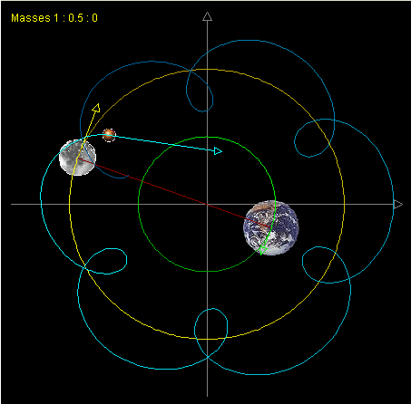
Many mathematicians have proofed that it is impossible to find a closed-form solution for n-body problem analytically[2][3]. The system could become unstable very easily. However, the problem can be solved numerically. The most common approach is to iterate over a sequence of small time steps. Within each time step, the acceleration on a body is approximated by the transient acceleration in the previous time step. The transient acceleration on a single body can be directly computed by summing the gravity from each of the other N-1 bodies. While this method is conceptually simple and is the algorithm of choice for many applications, its O(N2).
The simulation of N-body system can be used from simulation of celestial bodies (gravitational interaction)to interactions of a set of particles (electromagnetic interaction).
Parallel N-body problem
As MIT professors Dimitri Bertsekas and John Tsitsiklis stated in their book "Parallel and Distributed Computation: Numerical Methods", parallel computers have provided an excellent platform for numerical analysis. In the N-body problem, since each particle will interact with others by the force of gravity, the simulation of N-body system is computationally expensive for large numbers of N. There a O(N2) interactions to compute for every iteration. Furthermore, in order to have a accurate result, the discrete time step must relatively small. Thus, there has been a huge interest in faster parallel algorithm for N-body problem.
Data-parallel Implementation
Barnes-Hut Tree (BH tree)
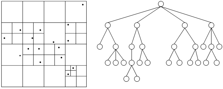
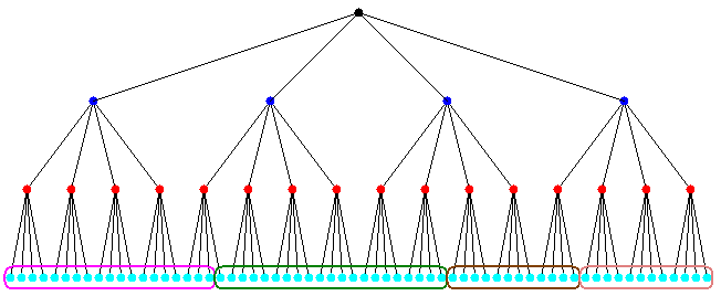
In 1985, Appel took the first step of decomposes the problem by introducing a tree structure[4]. In the next year, Barnes and Hut extend the tree-based force calculation with logarithmic growth of force terms per particle[5]. That is, construct a tree hierarchy(BH tree) of bodies based on the partition of entire space. The partition is shown on the left. The empty block have been pruned, thus the traversal time have been reduced fromO(N2) to O(N logN).
For each time step:
1. Build the BH tree.
2. Compute centers-of-mass bottom-up
3. For each body
   Star a depth-first traversal of the tree;
   Truncating the search at internal nodes where the approximation is applicable;
   Update the contribution of the node to the acceleration of the body.
4. Update the velocity and position of each body.
There are several challenges of this decomposition:
- Unlike the ocean current can be represented evenly by regular grid points in the entire space, the density of the galaxies is varying in different space. In some spaces the density of stars maybe very high, but in some other spaces there might be only few stars at certain time. This implies the computation load for each body will be different.
- The other challenge is that the position of the body is time-varying, which means the static assignment (which has been used in ocean application) may not work well.
- The force calculation of certain a body needs information from other bodies. In order to reduce the communication among processors, the partitions needs to be contiguous in any directions.
- The last challenge is that there is a trade-off between the level of decomposition and communication. That is, the fine grained approach could speed-up the force calculation but it will need more communications between different groups of stars.
Even though the Barnes-Hut tree decomposition algorithm have these challenges, BH tree is still the one of most efficient methods for solving the n-body problem.
Orthogonal Recursive Bisection (ORB)
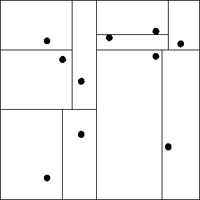
Unlike BH tree divided the space into square cells, the Orthogonal Recursive Bisection (ORB) divided space into rectangular with same number of bodies in each of them. It is a recursive approach because all processors are associated with the entire space at the very beginning; then a orthogonal line has been drawn to separate the space into bisection; each of the subsection has associated with half of the processors. Until the number of partition is equal to the number of processors.
Other Data-parallel Implementation
When using data-parallel algorithm to solve the N-body problem, one obvious approach for the data-parallel implementation is to divide the interactions into different sets based on the distances from current particle to other "interacting" particles. Thus the force from 'far away' particles can be updated less frequently or even can be ignored.
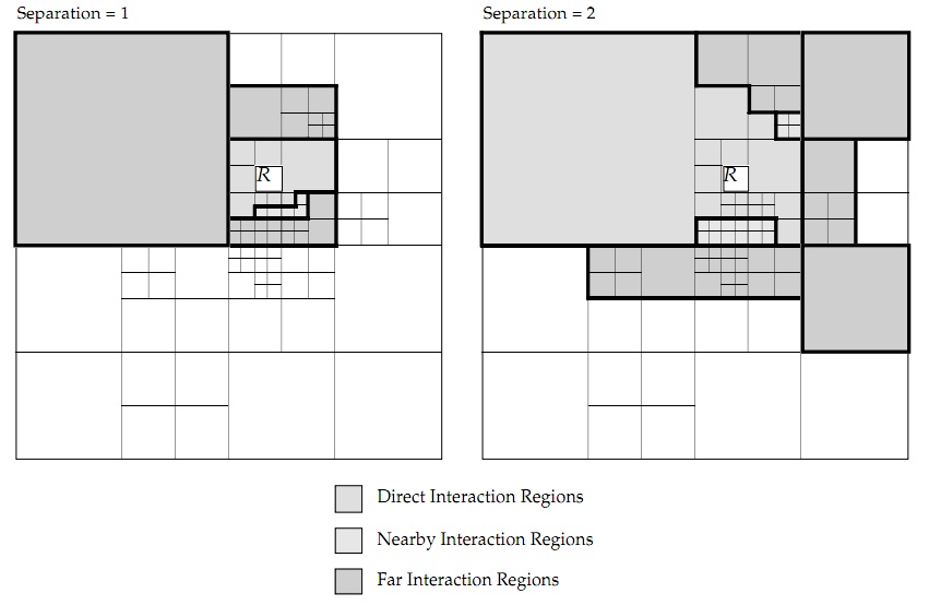
By separating the blocks by the Hamming distance to the R block. Three interaction list could be created by the distance: The direct interaction list Dr; the far interaction list Fr and the intermediate interaction list Hr
The steps for each iteration using the given decomposition of the simulation are [6]:
- Compute the multipole expansion coefficients for all leaves in the tree decomposition.
- Compute the multipole expansion coefficients for all internal nodes in the tree with depth ≥ 2.
- Compute the local expansion coefficients for a region R by summing R’s parent’s local expansion (shifted from the parent’s center to the center of R) with the sum of all of the multipole expansions in R’s far list, Fr(converting the multipole expansions to local expansions and shifting to the center of R) for all regions with depth ≥ 2.
- For each body, b, in each leaf region, R, compute all the direct forces on b from all the bodies in the regions in R’s direct interaction list (Dr).
- For each body, b, in each leaf region, R, compute the far force on b by evaluating the local expansion for region R at b’s position.
- For each body, b, in each leaf region, R, compute the intermediate force by evaluating the multipole expansion at b’s position for each region in R’s intermediate interaction list (Hr).
- Sum the 3 components of the force and potential for each body.
- Apply the forces, updating the positions and velocities, and move the bodies to their proper regions as indicated by boundary crossing.
Another data-parallel implementation can be found in [8]. The drawback of this type of approach is obvious: the error may be increased significantly due to the clustering process.
Costzones
It is easy to share the BH tree in a shared memory machine. The so-called Costzones is one of the approaches to implement the BH tree algorithm in the shared-memory machine. We know that the processor will accesses more the nearby bodies than distant ones. Since the BH tree already contain the spatial information of bodies (more likely the nearby bodies will have a same parent with me), the Costzones technique simply uses the data structure created by the BH tree.
The costzones method have a better performance in a shared-memory machine compared with the ORB method. The reason is mainly because the time spent in the space partition is shorter.
Besides the Costzones method of implementing the N-body simulation on shard-memory machines, there is a tremendous interests of using CUDA to solve the N-body problem by modern GPUs [10][11].
global void
calculate_forces(void *devX, void *devA)
{
extern __shared__ float4[] shPosition;
float4 *globalX = (float4 *)devX;
float4 *globalA = (float4 *)devA;
float4 myPosition;
int i, tile;
float3 acc = {0.0f, 0.0f, 0.0f};
int gtid = blockIdx.x * blockDim.x + threadIdx.x;
myPosition = globalX[gtid];
for (i = 0, tile = 0; i < N; i += p, tile++) {
int idx = tile * blockDim.x + threadIdx.x;
shPosition[threadIdx.x] = globalX[idx];
syncthreads();
acc = tile_calculation(myPosition, acc);
syncthreads();
}
// Save the result in global memory for the integration step.
float4 acc4 = {acc.x, acc.y, acc.z, 0.0f};
globalA[gtid] = acc4;
}
CUDA shows an impressive potential to execute extremely parallel applications such as N-body problem. Twenty years ago, the N-body simulation can only runs on super computers. Because of the development of CUDA makes the classical N-body problem become a term project for some graduate students (see 2008 Fall CS 525 Project2 n-body simulation in CUDA).
Message-passing Implementation
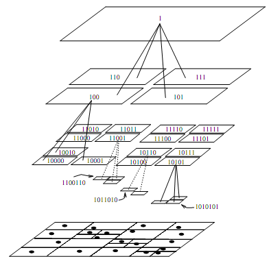
Implementing the BH tree algorithm is more difficult in a distributed-memory system compared with the shared-memory implementation. Because we need assign the different bodies to different processor dynamically. When the location of bodies have been changed exceed a certain limit, the BH tree needs to be reconstruct. The good news is we don't need reconstruct the BH tree very frequently(compared with the simulation step size).
In message-passing architectures, a processor’s local memory is often used as a software-controlled cache for communicated data, in addition to holding the processor’s own assigned data partition; that is, data are replicated in the memories of those processors that need to use them.
Warren and Salmon introduced a parallel hashed Oct-tree N-body algorithm[9]. The hashed Oct-tree is the message-passing version of BH tree implementation. One of the advantages of using hash table is that the non-local data may be accessed by requesting a key, which is a uniform addressing scheme and easy to be implemented on a message passing architecture. The pseudocode of tree traversal are shown below:
ListTraverse((*MAC)(hcell *))
{
copy root to walk_list;
while (!Empty(walk_list)) {
for (each item on walk_list) {
for (each daughter of item) {
if (MAC(daughter))
copy daughter to interact_list;
else
copy daughter to output_walk_list;
}
}
walk_list = output_walk_list;
}
}
There are two major challenges of using message-passing parallel to solve the N-body problem:
- The nonuniform and dynamic nature of the particle distribution, which implies that the partitions assigned to processors change with time to maintain load balancing and data locality;
- The need for long-range communication which is irregular as a result of the nonuniformity.
The typical message-passing strategy of allowing communicated data to accumulate in local memory and flushing them out at certain points in the program does not work well here like it does in regular predictable programs. Thus, the only convenient points at which to flush communicated data in the application program are the boundaries between computational phases. Since the amount of nonlocal data read from the tree during the force computation phase can be quite large, the memory overhead due to data replication can be large when replacement is managed in this typical message-passing style.
Other Parallel Approaches
Other than the conventional approaches, there are also some new techniques have been developed to simulate the N-body problem:
- Hardware side: The researcher in University of Tokyo have designed and built a special purpose hardware called GRAPE for the N-body simulation. The chip has been designed to optimize the computation of gravitational interactions.[12] The GRAPE has been keep developed by researchers, the most updated version is GRAPE 6.
- Software (algorithm) side: On the other hand, the high-level architecture-independent algorithms also have been develop to simulate the N-body problem[13]. These algorithm allowed researchers test their prototype parallel program under different architecture without using the machine-specified languages.
References
[1] Collection of remarkable three-body motions
[3] Diacu, F (01/01/1996). "The solution of the n-body problem" . The Mathematical intelligencer (0343-6993), 18 (3), p. 66.
[4] A. Appel, "An Efficient Program for Many-Body Simulation" , SIAM J. Scientific and Statistical Computing, vol. 6, 1985 (available at NCSU library)
[5] Barnes. Josh, Hut. Piet, (12/04/1986). "A hierarchical O(N log N) force-calculation algorithm". Nature (London) (0028-0836), 324 (6096), p. 446. (available at NCSU library)
[6] A Data-Parallel Implementation of the Adaptive Fast Multipole Algorithm 1993
[7] Johnsson, SL (01/01/1996). "A data-parallel implementation of hierarchical N-body methods". The international journal of supercomputer applications and high performance computing (1078-3482), 10 (1), p. 3.
[8] Implementing N-body Algorithms Efficiently in Data-Parallel Languages (1996)
[9] A Parallel Hashed Oct-Tree N-Body Algorithm (1993)
[10] N-Body Simulation using CUDA
[11] Fast N-Body Simulation with CUDA
[12] Tomoyoshi Ito, Junichiro Makino, Toshikazu Ebisuzaki, Daiichiro Sugimoto, A special-purpose N-body machine GRAPE-1, Computer Physics Communications, Volume 60, Issue 2, September 1990, Pages 187-194.
[13] Mills, P.H.; Nyland, L.S.; Prins, J.F.; Reif, J.H.; , "Prototyping N-body simulation in Proteus," Parallel Processing Symposium, 1992. Proceedings., Sixth International , vol., no., pp.476-482, 23-26 Mar 1992
[14] David E. Culler, Jaswinder Pal Singh and Anoop Gupta. "Parallel computer architecture : a hardware/software approach"Morgan Kaufmann Publishers, c1999.
Appendix: Comparison of Performance
The following table is a summary of sequential and parallel implementations of N-body simulation from [7].
| Author | Method and Error | Program Model | N | Times (s) | P | Efficiency | Machine |
| Salmon (1990) | BH, quadrupole | Message passing | ? | ? | ? | ? | Ncude |
| Warren_Salmon (1993) | BH,ϵ = 10-3 | Message passing | 8.78 M | 114 | 512 | 28% | Intel Delta |
| Warren_Salmon (1995) | BH,ϵ = 10-2 | Message passing | 2 M | 10.8 | 256 | ? | CM-5E |
| Liu-Bhatt (1994) | BH, quadrupole | Message passing | 10 M | 59 | 256 | 30% | CM-5 |
| Leathrum-Board(1992) | GR,p=8 | Shared memory | 1 M | 1520 | 32 | 20% | KSR-1 |
| Elliott-Board(1994) | GR,FFT,p=8 | Shared memory | 1 M | 1420 | 32 | 14% | KSR-1 |
| Schmidt-Lee(1991) | GR,p=8 | ? | 40,000 | 94 | 1 | 39% | CRAY Y-MP 8/864 |
| Zhao-Johnsson(1991) | Zhao, p=3 | Data parallel | 16,000 | 5 | 8 K | 12% | CM-2 |
| Hu-Johnsson | Anderson | Data parallel | 100 M | 180 | 256 | 27%-35% | CM-5E |
| Singh et al.(1993) | GR, 2-D, adaptive | Shared memory | ? | ? | ? | ? | DASH, KSR-1 |
All performance numbers are for uniform particle distributions. Methods used are for 3-D, unless other wise stated. "?" imply unavailable data.