File:GraphicalFigure9.png

Graphical Programming: Why? The history of computer programming languages is a continuous trend towards ever more powerful abstractions. Languages tend to push complexity into the background, letting the programmer focus primarily on the logic of the application.

While computer science abstractions are extremely useful, applying them in an engineering context can be particularly difficult for the uninitiated. As a way of managing program complexity, a number of companies have developed languages where graphics, rather than words, convey to the programmer’s intents to the computer. The power of images as abstractions is obvious in our age of increasing multi-media, and while there are very old (relatively speaking) graphical programming languages, the field is still relatively sparse.

Why this scarcity of graphical languages? We can not say. In our view the chief advantage of a graphical language is program control “lives” in the spatial structure of the code, rather than in the grammar. For grammar oriented individuals, and those used to programming languages, this may seem a disadvantage, however, for those more visual oriented, the two-dimensional space proffers a richer palette for creating. The following discussion illustrates how various abstractions are implemented in a few graphical languages. The elegant implementations of threading, of programming to interfaces, of refactoring for simplicity, and maintenance of type correctness are powerful reasons for engineers and computer scientist alike to utilize graphical means for creating code.

Representative Languages <describe the languages we will talk about, what they are used for, and the advantages they bring to their domains>

Throughout the web there are numerous definitions of object orientation [1,2,3]. In this discussion we hold the perspective that polymorphism, encapsulation, and inheritance are the core elements of an O-O language or system.

In the following sections we will explore each language described above from the perspective of the salient characteristics necessary for a language to be classified as object-oriented. While some of these are more properly classified as systems rather than languages, evaluating them in context of the O-O languages concepts provides a relevant approach to understanding the benefits and limitations of each tool.

LabVIEW With little doubt, the dominant force in graphical programming is National Instruments LabVIEW. Developed in 1986 as a tool to communicate with lab instruments, it grew into a full-fledged programming language with extensive capabilities. The examples used in the discussion below are all from a real application.

Data Flow The dominant paradigm in LabVIEW programming is data flow. Unlike most languages where code execution is controlled by sequential commands or callbacks, in LabVIEW data flows along wires, and a code objects only execute when all its inputs receive data values – Figure 1.

Figure 1: Two blocks (functions) that initialize memory for image capture. Data flow is always from left to right. The right block only executes after it receives the outputs from the left block. In this case, all the inputs (blue and pink boxes) are constants.

Strongly Typed In the above figure, different wires have different colors and texture patterns. LabVIEW is a strongly typed language: each color and texture pattern denotes a different data type. A terminal to a function only accepts wires of the correct type: this property virtual eliminating data-type errors while programming, because a wire is “broken” if it is not connected properly.

Figure 2: (a) Floating window shows the inputs (left) and outputs (right) the “IMAQ ArrayToImage” function expects and generates. Double, blue lines are 2D arrays of integers, purple, textured lines are image references, yellow-and-brown line is a cluster (linked-list), and the double, orange line is a 2D array of doubles. (b) This block will not execute. (c) The same block with the correct type input will execute (also note that some inputs are optional).

Control Structure All the major control structures exist in LabVIEW, some taking on multiple forms. A few of the more common ones are shown below.

Figure 3: The large outside box is a while loop. All the contents of the box are executed each iteration. The box to the right is a for loop. The N in its upper left-hand corner is the number of times it is to run. In this case, the green wire is an array of Boolean values, and the “[]” symbol where the wire intersects the for-loop’s box indicates that the loop will run execute for each element of the Boolean array. The box inside the for loop is a case structure with two cases, true and false. The left image shows the contents of the true case, the right shows the false case. True versus false is selected via the element extracted from the Boolean array.

Programming to Interfaces In LabVIEW, a function is called a Virtual Instrument, or VI, harking back to the beginnings of the language as an instrument control tool. The advantage of the strongly-typed paradigm is that a function’s interface is automatically documented as soon as the programmer re-factors some functionality into a sub-VI. Each VI has a front panel, which is the function’s interface, and a back panel, which is the function’s implementation. Thus, with no coercion or behavioral training, programmers write code to interfaces rather than implementations.

Figure 4: (a) The back panel of a VI (a function), (b) The front panel for the same VI, (c) the interface documentation automatically crated for the function.

Debugging The data flow paradigm automatically structures the code as it is written, regardless of the physical orientation. If you turn on the “highlight execution” option, debugging is trivial, as you can physically see the data flowing. Additionally, if you open a sub-VI, the data going into that sub-VI is shown on the front panel: after the program stops that data is still there, and you can re-run the VI with those values – an especially useful tool in complex applications where a function’s initial conditions are hard to derive.

Figure 5: Same function as Figure 4, but in debug mode. Note the small pop-up blocks showing the values in various wires, and the red dots indicating which inputs to the blocks already have their values. When executing, small indicators follow the path of the wires, graphically showing the data “flow.”

Encapsulation Throughout LabVIEW, data is encapsulation by the declaration of the controls and indicators on each VI’s front panel. A control is data that enters a function. An indicator is data that leaves a function. A typedef defines a container of data via a standalone front panel: controls, indicators, and constants may then be instantiated referencing that typedef. A modification to the typedef propagates through the whole application.

Figure 6: (a) A complex typedef (this one is viewed as an indicator, the control appears similar). (b) The structure of the typedef is apparent either by viewing the nesting of the boxes in (a), or by viewing the tree structure in (b). In either case, the head item, “glove data”, is a cluster; items (1)-(4) are also clusters, each containing four Booleans; 1d, 2d, and vec are clusters, each containing two doubles. This complex data is passed to many parts of the application.

While there are a host of data structures in LabVIEW, the principle ones are highlighted below: - Numeric: a number, can be integer, double, single, byte, etc., - String: the same as in other languages, - Array: can hold a collection homogenous of objects (including clusters), - Cluster: a form of a linked list that can hold a heterogeneous collection of other types, including other clusters. Example of these data types are shown below. Note that in the back panel the different data types are identified by their coloration and texture.

Polymorphic The triangular equal sign in Figure 7 is possibly the best example of LabVIEW’s polymorphic capabilities. The pinkish wires going into the equal sign are of the type shown in Figure 6. The equal block deals with it perfectly

Figure 7: An excerpt from Figure 3. The default equal function does the appropriate operations on all the elements of the pinkish wire. The pinkish wire’s type is that shown in Figure 6!

Multi-Threading Unlike traditional languages where threading is a difficult concept, in LabVIEW it is trivial. The example below shows a portion of the large application from which all the examples were drawn. There are no less than 10 threads shown. Multiple other’s exist in the application. Various mechanisms for inter-thread communication are used in the application, including polling, broadcasting, global variables, and queuing. Communication method is careful chosen based on program requirements.

Figure 8: Many threads. Each block not contained in or wired to a control structure is an independent thread.

Inheritance To this point we have not talked about inheritance. In general LabVIEW programming, inheritance is not necessary (the authors have never found reason to use it in years of programming), however it is robustly supported. Reference [5] is a fine overview of LabVIEW’s inheritance implementation, while [6] provides an excellent discussion of how LabVIEW’s designers chose their particular approach to inheritance, pass-by-value versus pass-by reference, and a host of other detailed computer-science questions.

Compiled Unlike many other languages, LabVIEW applications are actually compiled before they are run. When first introduced to the language, one usually suspects it is a scripting language however, as the compilation takes a mere fraction of a second.

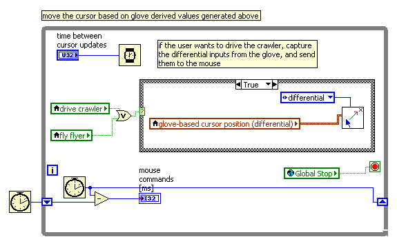
Weaknesses In practice, the primary weakness of LabVIEW’s graphical programming paradigm is by-reference programming. LabVIEW is designed as a value-passing language [6], and thus program clarity suffers when by-reference programming is necessary. An example is shown below. Note that the language still offers by-reference functionality, it is simply harder for the programmer to understand what is happening.

Figure 9: In the code above, the green and brown boxes are reference to front-panel controls. This is a polling loop that reads the values of the controls. Where it a loop that wrote to these same reference, and it was not the only piece of code that did so, steps to arbitrate writes would be required.

Other Features The LabVIEW tool suite is exceptional in a number of other ways. - It is easy to call dynamic libraries from with the language. - The same LabVIEW code (with certain exceptions) can be target to Windows, Mac, and Linux operating systems. What is more impressive is that the same code can be targeted at a hard real-time operating system, or turned into VHDL and sent to an FPGA. - By dropping in a special block, LabVIEW can directly execute MATLAB- and C-syntax code, or (using another block) directly call the MATLAB API. - Because the code is graphical and flows from left to right, large programs tend to flow off the screen. The programmers tendency is to keep the code in one screen however. This tendency promotes excellent refactoring practice, as programmers tend to collect sprawling pieces of code and put them into sub-Vis, thus keeping the high-level application clean.

<include an embedded link for all the above>

References [1] O-O Wiki: http://en.wikipedia.org/wiki/Object-oriented_programming [2] What is “Object-oriented programming”?, Bjarne Stroustrup, 1991 http://www.scribd.com/doc/21007168/Bjarne-Stroustrup-What-is-Object-Oriented-Programming-Allfreebooks-tk [3] PC Magazine O-O definition: http://www.pcmag.com/encyclopedia_term/0,2542,t=object-oriented+programming&i=48238,00.asp [4] The benefits of programming graphically in NI LabVIEW: http://www.ni.com/labview/whatis/graphical-programming/ [5] Inheritance in LabVIEW: http://zone.ni.com/reference/en-XX/help/371361B-01/lvconcepts/creating_classes/ [6] The decisions behind LabVIEW’s O-O design: http://zone.ni.com/devzone/cda/tut/p/id/3574